

Introduction
Today, we are thrilled to announce PAN 2, a foundation world model for physical intelligence.
Much of what makes an AI system intelligent with language comes from its ability to predict the next word. Physical intelligence, competence in acting in the physical world, rests in the same way on predicting the next world, or simulating how it will change in response to actions. Catching a ball requires anticipating contact and timing; pouring a cup of coffee, the physics of liquid flow; and stepping around a passer-by, the trajectory of another person across viewpoints. A system’s physical intelligence thus lies not in the abstract quality of its representations or the dexterity of its actions alone, but in how faithfully it can simulate the consequences of those actions. These simulations must produce observations that can be checked against the real world.
We call a model with this ability a world model, and it enables simulative reasoning, where an agent imagines the outcomes of its candidate actions before choosing among them. The more faithful the simulation, the closer those choices come to the right ones in the real world, and the more an agent can learn and plan without costly, slow or irreversible physical trials. To be useful, the simulated futures must be physically plausible sequences of consequences rather than renderings of whatever outcome that was requested. What it means to simulate the world well can be broken down into six dimensions of physical intelligence (6D-PI), from obeying the laws of physics to keeping the world moving on its own (see Evaluating World Models).
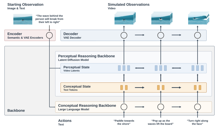
PAN 2 is designed to deliver this simulation at scale. It follows the Generative Latent Prediction (GLP) architecture, which learns latent world states through supervision on the next observations they reconstruct. A large language model (LLM), the conceptual reasoning backbone, predicts the next world state as a structured, time-grounded description of who acts, when, and how the camera moves. A latent diffusion model (LDM), the perceptual reasoning backbone, then predicts the perceptual detail that language leaves open, such as contact, deformation, and motion. An external agent can compare these simulated outcomes, revise plans, and choose what to execute, with new observations informing subsequent reasoning.
We build PAN 2 by coupling a pretrained LLM for conceptual reasoning with a perceptual reasoning backbone that we train from scratch on diverse real-world footage, and designing the text-based state representation that connects them. Its simulations must preserve action timing, physical interactions, and spatial coherence. This motivates PAN 2’s grounding in time, physics, and space.
Grounded in time, physics, and space
Explore all three themes: Time, Physics, and Space.Select a card to watch its video and browse individual examples.
Time-grounded actions. In the physical world, timing affects outcomes. The same press of the brake can stop a car short or end in a collision, depending on when it comes. The conceptual reasoning backbone (LLM) ties each world state and agent action to a precise timestamp, so the timing and order of actions are explicit for simulation. Each simulation builds on the outcome before it, so consequences carry forward: a car that swerves to avoid one obstacle faces the road from a new position, and every later decision starts from there.
Physics-grounded dynamics. A ball bounces, a glass shatters, a tablecloth drapes, and coffee splashes. A useful simulation must get each of these right, not just make them look convincing. The perceptual reasoning backbone (LDM) refines text and video representations together through joint attention. Supervision from real-world footage grounds these predictions in realistic motion, contact, and material changes.
Space-grounded viewpoint controls. To reason and plan, an agent needs a reliable model of the space it acts in, not merely a view of it. Training on videos with geometry-derived camera annotations teaches PAN 2 how viewpoint relates to scene geometry. This supports timed, language-specified camera movements while keeping viewpoint changes separate from object motion, like a soccer player looking up for a teammate while the ball keeps rolling.
How PAN 2 compares
PAN 2 is built for AI agents to use, so we judge it mainly by automated checks of what its simulations show. We build our own test cases for the six dimensions of physical intelligence (6D-PI) and for multi-step plans (see Evaluating World Models), and complement them with public physics (Physics-IQ) and robotics (RBench) benchmarks. PAN 2 completes 75.1% of individual steps and 34.0% of full plans, achieving the highest full-plan completion among the models we studied while remaining competitive on single actions across the six dimensions. It would also rank first among open models and third overall on Physics-IQ Verified in the public leaderboard setting. We also assess simulation quality through blinded human comparisons based on action adherence, physical plausibility, and world consistency. PAN 2 ranks second among the four evaluated open models.
About these results
We compare PAN 2 with the open models Cosmos 3 Super, LTX-2.5 and MiniMax-H3, and the closed models FLUX 3 and Seedance 2.5. Each plot uses its own labeled scale, and higher is better throughout. †Closed models, generated once; blocked or unreturned videos are excluded.
Single-action evaluation pools judged questions on the six dimensions across image-to-video and text-to-video; multi-step plan evaluation pools full-plan completion across both text-to-video and image-to-video. Physics-IQ uses submitted leaderboard configurations, where FLUX 3 uses Claude Opus 5.5 prompts without best-of-N, and PAN 2 uses Claude Opus 5.5 as its conceptual reasoning backbone. RBench uses Cosmos 3 Super’s Reasoner, MiniMax-H3’s official prompt skill with Kimi-K3, and PAN 2 with GPT-6 Astra as its conceptual reasoning backbone.
For human judgment, reviewers compared simulations side by side, without knowing which model made them, and chose the better one or a tie based on action adherence, physical plausibility, and world consistency; Bradley–Terry fits turn these choices into Elo ratings. PAN 2 uses GPT-6 Astra as its conceptual reasoning backbone.
Architecture
How does PAN 2 turn an action instruction into a simulated future? The answer lies in how it splits reasoning from rendering. The PAN 2 architecture comprises an encoder, a backbone that reasons by predicting the next state, and a visual decoder that renders that state into the next observation. Formally, PAN 2 models the next observation, a video, given the current observation (an optional image with text) and an action (an instruction in text with the duration to simulate), through estimated latent states, as shown in the equation below:
From reasoning to simulation
The encoder represents the starting observation in two ways: the vision encoder of a pretrained vision-language model captures its conceptual content, while a VAE encoder preserves perceptual detail as video latents. The conceptual reasoning backbone, an LLM, uses the observation and the action to predict a text-based next state comprising global scene attributes and time-grounded events. The perceptual reasoning backbone, an LDM implemented as an MMDiT, uses this text-based state and optional starting-frame latents to predict video latents over a window of up to 20 seconds. The VAE decoder renders these latents into observation frames. The text-based state serves as the intermediate representation between the two backbones: the LLM reasons explicitly about events, actions, and camera motion, while the LDM predicts the perceptual details the description leaves open.
Both backbones operate on latent states, with the perceptual state decoded into observations. Supervision on these generated observations grounds latent-state learning in the observed world.
Evaluating World Models
A simulation can look right and still be wrong. A door may swing open before it is unlocked, or the camera may barely turn when asked to look behind. Metrics of video quality don’t catch this, so we built our own test cases, organized around the six dimensions of physical intelligence: physical consistency, causal coherence, entity persistence, constraint satisfaction, viewpoint invariance, and objective dynamism. Together, they ask whether simulations obey physical laws, follow actions in order, preserve entities and their states, respect action prerequisites, keep the world unchanged as the camera moves, and keep the world moving beyond the agent’s actions. We run them in two studies, single actions and multi-step plans; a VLM judge answers yes/no questions about each simulation, and VGGT-Ω verifies camera motion from estimated geometry.
Select a study to see how one simulation is scored.
Single actions ask whether a simulated action produces consequences consistent with the six dimensions. Each test case gives a starting observation (an optional image and text) and an action, covering image-to-video and text-to-video; most test several dimensions at once.
How it’s scored
We use VLM judges to answer one action question and one question for each dimension the test case is tagged with, and use VGGT-Ω to evaluate camera movements. Action completion gates only the designated persistence checklist questions, rather than every dimension. Scores pool passed questions over judged questions, excluding unclear answers. For viewpoint invariance, the geometric check measures whether the camera follows the command, as most benchmarks do; whether the world stays unchanged as it moves is tested in part through entity persistence.
Example LTX-2.5, I2V, seed 125
start image + prompt
The hand pours all of the juice from the wide tumbler into the tall narrow glass and sets the empty tumbler back down.
tagged: Constraint satisfaction, Physical consistency, Objective dynamism
0.2 stumbler full, glass empty
Judge verdictJudge
Single-action walkthrough
Hover or tap a check to see its question, evidence and verdict.
Start image + prompt
The hand pours all of the juice from the wide tumbler into the tall narrow glass and sets the empty tumbler back down.
Tagged: Constraint satisfaction, Physical consistency, Objective dynamism.
Generated video LTX-2.5, I2V, seed 125
The hand should pour all of the juice into the tall glass and set the empty tumbler back down.
Four segments (0–1.9, 1.9–6.4, 6.4–7.75, 7.75–10 s), labelled by their poster frames at 0.2, 3, 7 and 9.5 s. Click a frame to play its segment.
Objective dynamism VLM judge
- Question
- Does the hand pour juice from the wide tumbler into the narrow glass?
- Evidence
- Judge: the hand tilts the wide tumbler over the narrow glass and a stream of orange juice flows from it into the narrow glass, from about 1.9 s to 6.4 s.
- Verdict
- pass matches expected
Physical consistency VLM judge
- Question
- Does the juice stand much higher in the narrow glass than it did in the wide tumbler?
- Evidence
- Judge: at 0.2 s the juice fills only about two-thirds of the short wide tumbler, while by 7 s the same juice stands near the rim of the much taller narrow glass, a far higher level.
- Verdict
- pass matches expected
Constraint satisfaction VLM judge
- Question
- Does all of the juice end up in the tall narrow glass?
- Evidence
- Judge: after the pour, the hand sets the wide tumbler back down at about 9.1–9.8 s and it is still full of orange juice, so not all of the juice ended up in the narrow glass. The tall glass is full too, so the juice has been duplicated rather than moved.
- Verdict
- fail does not match expected
Dimension checks passed: 2/3
The pour is shown, so objective dynamism passes; the juice stands much higher in the narrow glass, so physical consistency passes; the tumbler is set back down still full, so not all of the juice ended up in the tall glass and constraint satisfaction fails. The scenario scores 2/3.
Multi-step plans ask whether the dimensions hold throughout a plan, rather than only at its final outcome. Each test case presents an everyday task with 3–6 ordered steps over 20 seconds, posed in both image-to-video and text-to-video and simulated in one pass. We report step completion, the mean share of steps completed per simulation, and full-plan completion, the share of simulations that complete every step.
How it’s scored
Every step is judged separately and checked for temporal order; each positive decision must survive five skeptical re-checks, and steps involving camera movements also require geometric verification. Simulating the full plan in one pass tests faithful multi-step next-world prediction, with closed-loop plan selection left to the agent that uses the model.
Example Cosmos 3, T2V, seed 123
T2V prompt (shortened)
“…Her orange kite is caught in the branches of the tree above you, too high to reach, and a long bamboo pole lies on the grass behind you. Free the kite and give it back to the girl.”
S1Look up to the kite in the tree
Judge verdictJudge Qwen3.8-27B: pass 1 says yes, then 5 skeptic re-asks must all say yes; camera steps also need VGGT. A step is done only if every check passes.
Multi-step plan walkthrough
Hover or tap a step card to see its pass-1 answer, skeptic re-asks, VGGT check and the decision.
T2V prompt shortened
“…Her orange kite is caught in the branches of the tree above you, too high to reach, and a long bamboo pole lies on the grass behind you. Free the kite and give it back to the girl.”
The task has six ordered steps, S1–S6; each is judged separately.
Simulation Cosmos 3, T2V, seed 123
One segment of the simulation per step, cut where the step's action (or the failed attempt) is on screen; the thumbnail and the time under it are the judge's timestamp for that step (0.0, 7.8, 10.8, 14.1, 16.1 and 18.6 s). Click a frame to play its segment.
Pass 1 VLM
Qwen3.8-27B asks one yes/no question per step. It says yes for all six.
Skeptic ×5 VLM
Every yes is re-asked five times by a skeptic prompt, and all five must say yes. S1, S2, S3, S5 and S6 get 5/5; S4 (push the pole against the kite) gets only 3/5.
VGGT camera trajectory
Camera steps also need geometric confirmation from VGGT. S1: no tilt up. S2: the camera only turns 11°. S3–S6 are not camera steps (–).
S1 Look up to the kite in the tree judge time 0.0 s · segment 0.00–6.75 s
- Pass 1
- yes
- Skeptic ×5
- 5/5
- VGGT
- no tilt up
- Step
- not done Pass 1 and all five skeptics say yes, but VGGT finds no upward tilt of the camera.
S2 Turn around to the bamboo pole judge time 7.8 s · segment 6.75–8.25 s
- Pass 1
- yes
- Skeptic ×5
- 5/5
- VGGT
- turns 11°
- Step
- not done Pass 1 and all five skeptics say yes, but VGGT measures only an 11° turn.
S3 Pick up the bamboo pole judge time 10.8 s · segment 8.25–11.50 s
- Pass 1
- yes
- Skeptic ×5
- 5/5
- VGGT
- – not asked
- Step
- done Pass 1 says yes and all five skeptic re-asks agree; no camera check is needed.
S4 Push the pole against the kite judge time 14.1 s · segment 11.50–15.25 s
- Pass 1
- yes
- Skeptic ×5
- 3/5 2 of 5 say no
- VGGT
- – not asked
- Step
- not done Pass 1 says yes, but two of five skeptic re-asks say no, so the step is not done.
S5 The kite comes out of the tree judge time 16.1 s · segment 15.00–16.75 s
- Pass 1
- yes
- Skeptic ×5
- 5/5
- VGGT
- – not asked
- Step
- done Pass 1 says yes and all five skeptic re-asks agree; no camera check is needed.
S6 Hand the kite to the girl judge time 18.6 s · segment 16.75–20.04 s
- Pass 1
- yes
- Skeptic ×5
- 5/5
- VGGT
- – not asked
- Step
- done Pass 1 says yes and all five skeptic re-asks agree; no camera check is needed.
Step completion: 3/6 = 50%
VGGT rejects the upward look (no tilt) and the turn to the bamboo pole (only 11°), and two of five skeptic re-asks reject the push against the kite. Three of six steps are done: 50% step completion.

Full plans compound on single steps
Across all six models, full-plan completion is lower than step completion because errors accumulate across a plan. The results follow a single compounding curve (R² = 0.986): as individual steps become more reliable, each improvement yields a larger gain in full-plan completion. The fitted curve suggests that raising step completion from 75% to 90% would roughly double full-plan completion, from one-third to two-thirds.
Show as table
| Model | Step completion | Full-plan completion |
|---|---|---|
| MiniMax-H3 | 75.1 | 32.5 |
| PAN 2 | 75.1 | 34.0 |
| FLUX 3 | 72.4 | 26.8 |
| Seedance 2.5 | 69.0 | 24.5 |
| Cosmos 3 Super | 47.7 | 9.5 |
| LTX-2.5 | 38.5 | 4.0 |
What we learned. All six models we studied fall on a single curve, where full-plan completion is a power-exponential function of step completion. Today’s leading world models sit where that curve turns steep. As individual steps become more reliable, we expect rapid gains in full-plan simulation that resemble capability emergence, bringing simulative reasoning within reach.
Technical Details
Building a world model for simulative reasoning requires answering several key technical questions: where language ends and the latent begins, what kind of data to learn dynamics from, what training on data alone misses, and how to train efficiently at scale. In this section, we examine each decision and its measured consequences.
Where does language end and the latent begin?
The text-based state defines the division of work between PAN 2’s two backbones. The LLM reasons about the conceptual content of the next state, and the LDM fills in the perceptual details left open by the text-based state. In PAN 2, we make subjects, the timing of events and actions, and camera motion explicit, while leaving geometry, appearance, and the fine details of motion to the LDM. This choice raised two questions.
Is the LLM doing more than tidying the prompt? Many video generators already put an LLM in front of a diffusion model to rewrite prompts. To see whether PAN 2’s conceptual backbone does more, we kept the LDM fixed and varied the level of conceptual reasoning by PAN 2’s LLM: none (the action instruction goes directly to the LDM), format-only (the LLM rewrites the input into the structured format without reasoning), or full (the LLM reasons about how the world will evolve and writes a complete text-based state).
Show as table
| Conceptual reasoning | Single actions: six dimensions | Multi-step plans: step completion | Multi-step plans: full-plan completion |
|---|---|---|---|
| None (action only) | 45.1 | 8.7 | 0.0 |
| Format | 78.2 | 70.7 | 27.8 |
| Full | 84.6 | 75.1 | 34.0 |
Without conceptual reasoning, the model’s single-action score drops by nearly half and full-plan completion falls to zero, showing the LDM alone is insufficient for reasoning about the timing, events, and camera motion required for simulating action sequences. Format-only reasoning recovers most of the single-action gap but only part of the multi-step gap, confirming that the depth of conceptual reasoning, not just input formatting, is what drives plan simulation.
What we learned. Conceptual reasoning is integral to PAN 2’s simulation, helping actions, events, and camera movements unfold in the right order and at the right time. We expect advances in their LLM components to further improve the simulation capabilities of world models.
How should the states be written? We train the LDM on the same structured state descriptions it receives from the LLM at inference, aligning its training and test-time inputs. Each training clip is therefore paired with a structured JSON caption comprising two components. Global scene attributes capture the initial scene and subject identities, along with persistent context such as lighting, viewing perspective, and visual style. Time-grounded events describe subject actions, observed changes in object and scene states, and camera movements over explicit time intervals. This structure makes subjects, action timing, and camera motion explicit in the states the LDM learns to simulate.
We generate these annotations in three stages, which the example below steps through: a temporal scaffold, in which a vision–language model (VLM) marks when events and actions happen; camera evidence, in which estimated geometry gives the camera motion (VGGT-Ω); and caption synthesis, in which a VLM combines the two and adds detailed descriptions to produce the final structured caption.
How the captions are generated
- Temporal scaffold. A VLM identifies event boundaries and finer-grained action intervals from timestamped frames.
- Camera evidence. VGGT-Ω estimates camera parameters. Deterministic rules convert changes in translation, rotation, and field of view into event-aligned motion labels.
- Caption synthesis. A VLM combines video frames with the temporal scaffold and geometry-derived camera plan to produce a structured caption, associating actions with subjects and describing observed state changes. For matched events, the geometric plan determines the caption’s camera-motion field.
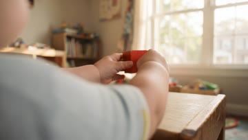
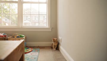
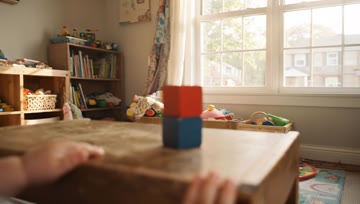
Select a block below to inspect it.
subjects_lifecycleA worn wooden tabletop fills the lower half of the view. A red cube stands to the left of a blue cube near the middle of the table, with a gap between them.…
A worn wooden tabletop fills the lower half of the view. A red cube stands to the left of a blue cube near the middle of the table, with a gap between them. Two small hands rest at the near edge. Low wooden shelves with toys, baskets and books stand in the left background. A large white-framed window occupies the upper right, with patterned curtains beside it and a toy-filled basket below.
- Style
- Photorealistic continuous shot
- Lighting
- Window daylight, warm tones, soft shadows
- View
- Low viewpoint just behind the child at table height. Hands and forearms occupy the foreground; a pale sleeve, shoulder and the side of the head enter the left foreground during stacking.
- Style
- Photorealistic continuous shot
- Lighting
- Window daylight, warm tones, soft shadows
- View
- Low viewpoint just behind the child at table height. Hands and forearms occupy the foreground; a pale sleeve, shoulder and the side of the head enter the left foreground during stacking.
The hands reach around the red cube, lift it clear of the tabletop and position it over the blue cube. The red cube is lowered onto the blue cube and…
The hands reach around the red cube, lift it clear of the tabletop and position it over the blue cube. The red cube is lowered onto the blue cube and released. The hands withdraw, leaving an upright two-block tower, red above blue, near the middle of the table.
grips .
places on .
releases and withdraws.
reaches for and grips .
lifts and places it on top of .
releases and withdraws from the tower.
The table and tower leave the view, revealing carpet, the edge of a patterned play mat, a toy basket below the window and the wall to its right. A ginger cat…
The table and tower leave the view, revealing carpet, the edge of a patterned play mat, a toy basket below the window and the wall to its right. A ginger cat is seated beside the white baseboard near an electrical outlet, visible from about 3.7 seconds. After sitting upright, it lowers its head toward its forepaws and the carpet, shifts its front paws and crouches close to the wall. Near the end of the interval its head starts to rise again.
sits beside the baseboard.
lowers its head and shifts its front paws.
crouches with its head near the carpet.
starts to raise its head.
sits upright beside the baseboard.
lowers its head toward its forepaws and shifts its front paws.
crouches with its head close to the carpet beside the wall.
starts to raise its head.
The cat raises its head and settles upright facing toward the table. It remains briefly visible by the wall as the table and two-block tower come back into…
The cat raises its head and settles upright facing toward the table. It remains briefly visible by the wall as the table and two-block tower come back into view, then passes out of the right edge around 9.4 seconds. The tower remains upright with red on blue; the hands rest along the near table edge. The final view holds on the unchanged stack, with the window and toy shelves in the background.
raises its head and sits upright.
remains seated.
rests below stacked on .
raises its head and settles upright facing toward the table.
remains seated beside the baseboard.
rests at the near table edge below the unchanged stack of on .
Description
The hands reach around the red cube, lift it clear of the tabletop and position it over the blue cube. The red cube is lowered onto the blue cube and released. The hands withdraw, leaving an upright two-block tower, red above blue, near the middle of the table.
Actions
reaches for and grips .
lifts and places it on top of .
releases and withdraws from the tower.
Description
The table and tower leave the view, revealing carpet, the edge of a patterned play mat, a toy basket below the window and the wall to its right. A ginger cat is seated beside the white baseboard near an electrical outlet, visible from about 3.7 seconds. After sitting upright, it lowers its head toward its forepaws and the carpet, shifts its front paws and crouches close to the wall. Near the end of the interval its head starts to rise again.
Actions
sits upright beside the baseboard.
lowers its head toward its forepaws and shifts its front paws.
crouches with its head close to the carpet beside the wall.
starts to raise its head.
Description
The cat raises its head and settles upright facing toward the table. It remains briefly visible by the wall as the table and two-block tower come back into view, then passes out of the right edge around 9.4 seconds. The tower remains upright with red on blue; the hands rest along the near table edge. The final view holds on the unchanged stack, with the window and toy shelves in the background.
Actions
raises its head and settles upright facing toward the table.
remains seated beside the baseboard.
rests at the near table edge below the unchanged stack of on .
View full caption
Subjects
Initial frame
A worn wooden tabletop fills the lower half of the view. A red cube stands to the left of a blue cube near the middle of the table, with a gap between them. Two small hands rest at the near edge. Low wooden shelves with toys, baskets and books stand in the left background. A large white-framed window occupies the upper right, with patterned curtains beside it and a toy-filled basket below.
Clip context
- Style
- Photorealistic continuous shot
- Lighting
- Window daylight, warm tones, soft shadows
- View
- Low viewpoint just behind the child at table height. Hands and forearms occupy the foreground; a pale sleeve, shoulder and the side of the head enter the left foreground during stacking.
event_description
The hands reach around the red cube, lift it clear of the tabletop and position it over the blue cube. The red cube is lowered onto the blue cube and released. The hands withdraw, leaving an upright two-block tower, red above blue, near the middle of the table.
contained_actions
reaches for and grips .
lifts and places it on top of .
releases and withdraws from the tower.
event_description
The table and tower leave the view, revealing carpet, the edge of a patterned play mat, a toy basket below the window and the wall to its right. A ginger cat is seated beside the white baseboard near an electrical outlet, visible from about 3.7 seconds. After sitting upright, it lowers its head toward its forepaws and the carpet, shifts its front paws and crouches close to the wall. Near the end of the interval its head starts to rise again.
contained_actions
sits upright beside the baseboard.
lowers its head toward its forepaws and shifts its front paws.
crouches with its head close to the carpet beside the wall.
starts to raise its head.
event_description
The cat raises its head and settles upright facing toward the table. It remains briefly visible by the wall as the table and two-block tower come back into view, then passes out of the right edge around 9.4 seconds. The tower remains upright with red on blue; the hands rest along the near table edge. The final view holds on the unchanged stack, with the window and toy shelves in the background.
contained_actions
raises its head and settles upright facing toward the table.
remains seated beside the baseboard.
rests at the near table edge below the unchanged stack of on .
{
"video_style": "Photorealistic continuous shot",
"lighting": "Window daylight, warm tones, soft shadows",
"perspective_view": "Low viewpoint just behind the child at table height. Hands and forearms occupy the foreground; a pale sleeve, shoulder and the side of the head enter the left foreground during stacking.",
"subjects_lifecycle": [
{
"subject_id": "",
"display_name": "Child's hands",
"subject_attribute": "Small light-skinned hands and forearms, with a pale blue short sleeve."
},
{
"subject_id": "",
"display_name": "Red wooden block",
"subject_attribute": "Red-painted wooden cube with slightly worn edges."
},
{
"subject_id": "",
"display_name": "Blue wooden block",
"subject_attribute": "Dark blue-painted wooden cube, similar in size to the red cube, with worn corners."
},
{
"subject_id": "",
"display_name": "Ginger cat",
"subject_attribute": "Small short-haired ginger tabby cat with darker stripes, a pale muzzle and chest, triangular ears and a long tail."
}
],
"init_frame_visual_description": "A worn wooden tabletop fills the lower half of the view. A red cube stands to the left of a blue cube near the middle of the table, with a gap between them. Two small hands rest at the near edge. Low wooden shelves with toys, baskets and books stand in the left background. A large white-framed window occupies the upper right, with patterned curtains beside it and a toy-filled basket below.",
"events": [
{
"event_index": 0,
"time_range_sec": "0 to 3",
"event_description": "The hands reach around the red cube, lift it clear of the tabletop and position it over the blue cube. The red cube is lowered onto the blue cube and released. The hands withdraw, leaving an upright two-block tower, red above blue, near the middle of the table.",
"camera_motion": [
{
"time_range_sec": "0 to 3",
"camera_motion": [
"static"
]
}
],
"contained_actions": [
{
"time_range_sec": "0.3 to 0.9",
"action": " reaches for and grips ."
},
{
"time_range_sec": "0.9 to 2.4",
"action": " lifts and places it on top of ."
},
{
"time_range_sec": "2.4 to 2.8",
"action": " releases and withdraws from the tower."
}
]
},
{
"event_index": 1,
"time_range_sec": "3 to 8",
"event_description": "The table and tower leave the view, revealing carpet, the edge of a patterned play mat, a toy basket below the window and the wall to its right. A ginger cat is seated beside the white baseboard near an electrical outlet, visible from about 3.7 seconds. After sitting upright, it lowers its head toward its forepaws and the carpet, shifts its front paws and crouches close to the wall. Near the end of the interval its head starts to rise again.",
"camera_motion": [
{
"time_range_sec": "3 to 5",
"camera_motion": [
"pan_right"
]
},
{
"time_range_sec": "5 to 8",
"camera_motion": [
"static"
]
}
],
"contained_actions": [
{
"time_range_sec": "3.7 to 5.7",
"action": " sits upright beside the baseboard."
},
{
"time_range_sec": "5.7 to 6.5",
"action": " lowers its head toward its forepaws and shifts its front paws."
},
{
"time_range_sec": "6.5 to 7.8",
"action": " crouches with its head close to the carpet beside the wall."
},
{
"time_range_sec": "7.8 to 8",
"action": " starts to raise its head."
}
]
},
{
"event_index": 2,
"time_range_sec": "8 to 12",
"event_description": "The cat raises its head and settles upright facing toward the table. It remains briefly visible by the wall as the table and two-block tower come back into view, then passes out of the right edge around 9.4 seconds. The tower remains upright with red on blue; the hands rest along the near table edge. The final view holds on the unchanged stack, with the window and toy shelves in the background.",
"camera_motion": [
{
"time_range_sec": "8 to 9.75",
"camera_motion": [
"pan_left"
]
},
{
"time_range_sec": "9.75 to 12",
"camera_motion": [
"static"
]
}
],
"contained_actions": [
{
"time_range_sec": "8 to 8.5",
"action": " raises its head and settles upright facing toward the table."
},
{
"time_range_sec": "8.5 to 9.3",
"action": " remains seated beside the baseboard."
},
{
"time_range_sec": "9.5 to 12",
"action": " rests at the near table edge below the unchanged stack of on ."
}
]
}
],
"quality": {
"video_quality": "Hands and blocks are well resolved. Background objects are softly focused, with additional blur during the turns and bright highlights through the window.",
"text_logos_overlays": null,
"artifacts": {
"visual_quality_issue": false,
"black_border": false,
"blurred_sidebar": false,
"talking_head": false,
"watermark": false,
"template_or_text_dominated": false,
"edited_or_discontinuous": false,
"video_game": false,
"animation": false,
"ai_generated_content": false
}
}
}Click any component in the timeline to see its details.
We compared this format with two plain-text alternatives, one emphasizing diverse content and one following a fixed structure. Since a caption describes the conceptual state that the perceptual reasoning backbone expands on, we evaluated each format by how well an LDM trained on it predicts held-out videos, using validation loss. The JSON captions contained the most detail and yielded the lowest loss.
Show as table
| Caption recipe | Distinct claims per video | Held-out loss |
|---|---|---|
| JSON (structured) | 49.43 | 0.383243 |
| Plain text (diverse) | 45.97 | 0.385521 |
| Plain text (structured) | 41.04 | 0.386267 |
What we learned. By capturing more of the world’s complexity in text-based states, we leave less for the LDM to infer when simulating perceptual details. This improves prediction without increasing the LDM’s capacity.
Learning dynamics from the real world
A world model learns physical dynamics from the observations it is trained on, so we select data for real-world relevance rather than visual appeal. We filter video clips for motion and quality, deduplicate them, and balance them across a taxonomy of topics (expand Data taxonomy and balancing below for details).
We tested whether excluding synthetic content improves simulation quality. After the earliest phase of training, we exclude gameplay, animation, computer-generated renders, and simulation videos, so the model learns dynamics from the real world rather than from stylized approximations of it. We trained two 9B models for 40,000 steps, one with synthetic content and one without. In blinded comparisons based on action adherence, physics, and world consistency, the model trained without synthetic content won 58% of votes.
Show as table
| Data recipe | Share of votes (%) | Elo |
|---|---|---|
| Excluding synthetic content | 58.0 | 1528 |
| Default | 42.0 | 1472 |
What we learned. What we leave out of training data matters as much as what we put in. To learn faithful physical dynamics, a world model benefits from real-world observations rather than synthetic approximations.
Data taxonomy and balancing
We organize clips into a taxonomy of 12 meta-topics and 149 subtopics. Excluding synthetic content after the earliest phase of training leaves the 11 meta-topics and 138 subtopics shown below, with target allocations that account for concept coverage and available clean data. Within subtopics, we cluster caption embeddings into 1,988 families that capture finer variation in appearance and action. Within each allocation, selection favors perceptual detail, meaningful motion, and semantic diversity. Early training balances subtopics and duration; later training adds finer cluster-family control.
Camera & Ego-Motion
3 meta-topics · 40 subtopics- Navigation17 subtopics
- Driving & Transportation14 subtopics
- Aerial Exploration9 subtopics
Agents & Interaction
4 meta-topics · 44 subtopics- Human Motion13 subtopics
- Multi-Agent Interaction11 subtopics
- Animals10 subtopics
- Robotics10 subtopics
Objects & Physical World
4 meta-topics · 54 subtopics- Objects13 subtopics
- Object Manipulation14 subtopics
- Physical Dynamics15 subtopics
- Nature & Environment Dynamics12 subtopics
Synthetic content
Excluded from continued training onwardReward-based learning
After flow-matching training, the LDM still makes mistakes that its training objective doesn’t penalize directly (e.g., an object that vanishes mid-clip, or a hand that passes through the cup it’s grabbing). We thus refine it through reward-based learning on its own generated videos. Following RewardDance’s generative scoring principle, we use the frozen VisionReward model to answer 13 questions covering object structure and persistence, motion, composition, and perceptual detail, and use its answers to compute the reward. Over 600 steps, the total reward and each of its parts rise steadily.
Implementation details
The reward is a normalized weighted average of VisionReward’s yes probabilities, computed pointwise for each generated video.
For perceptual detail, we score native-resolution crops to capture fine texture and artifacts that downsampling can hide.
We adopt the ReFL algorithm, where reward gradients pass through the frozen reward model and VAE decoder to update the LDM, without backpropagating through the full rollout.
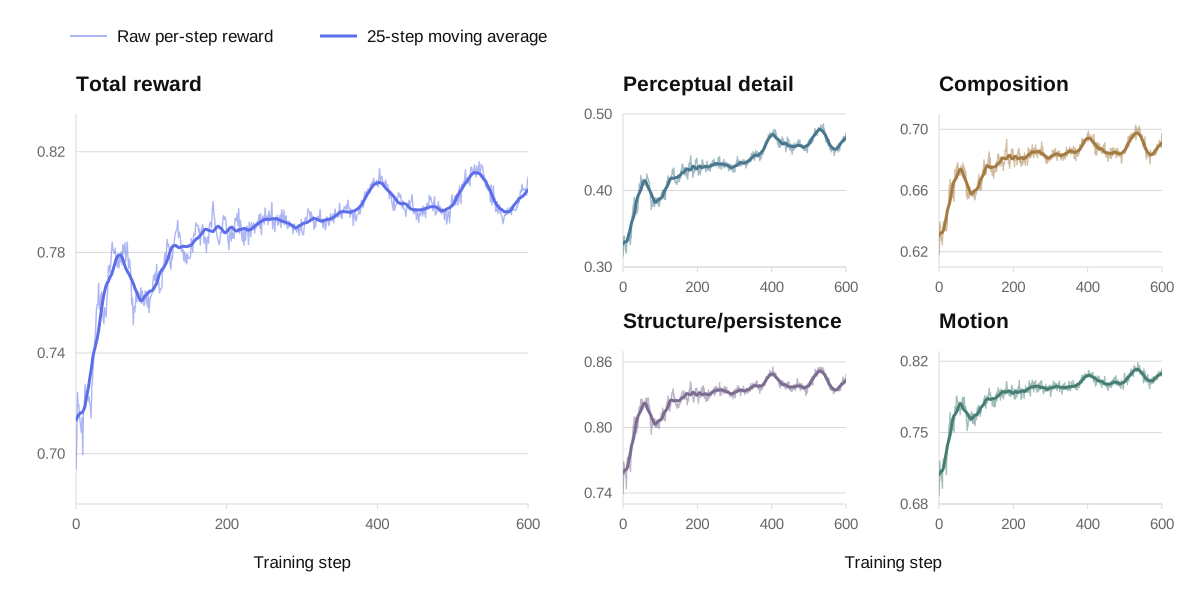
What does the reward actually change? Comparing the model before and after reward-based learning shows what a reward adds, and what it can cost. Causal coherence rose by more than eight points and full-plan completion by nearly four, even though the reward never scores the order of events. Viewpoint invariance and physical consistency, on which the reward offers little signal, went down.
Show as table
| After flow-matching training | After reward-based learning | Change | |
|---|---|---|---|
| Causal coherence | 78.8 | 87.3 | +8.5 |
| Entity persistence | 91.6 | 93.1 | +1.5 |
| Viewpoint invariance | 74.7 | 71.6 | −3.0 |
| Physical consistency | 77.7 | 75.1 | −2.5 |
| Constraint satisfaction | 82.8 | 82.8 | +0.1 |
| Objective dynamism | 92.3 | 92.4 | +0.2 |
| Overall (single actions) | 83.6 | 84.1 | +0.5 |
| Step completion | 71.3 | 74.1 | +2.8 |
| Full-plan completion | 28.2 | 31.8 | +3.7 |
Because a learned reward covers only part of what faithful simulation requires, we build our final model as a weighted average of the checkpoints before and after reward-based learning to retain its gains while mitigating reward hacking (model soups, rewarded soups).
What we learned. Reward-based learning complements flow matching by improving capabilities important for simulative reasoning, even when they are not directly rewarded. However, designing rewards that capture all aspects of faithful simulation and preventing reward hacking remain challenges, as they do for LLMs.
Scaling Flow Matching with Per-Head Muon
Training a 29B diffusion transformer from scratch requires an efficient optimizer. PAN 2 uses a hybrid optimizer built around per-head Muon.
Per-head Muon reshapes a momentum update so that a few high-energy directions do not dominate it. For attention, we split the Q/K/V update into head-sized matrices, run five Newton–Schulz steps on each head independently, and then reassemble the results. This lets each head balance its own update spectrum instead of being normalized as part of one large fused matrix. It does not force different heads to be orthogonal; they still interact through attention and the training objective.
Which parameters use which optimizer
Attention query, key, and value (Q/K/V) weights use per-head updates; attention-output and feed-forward weights, along with selected input and refiner projections, use matrix-wise Muon; the remaining parameters use AdamW. Biases, normalization, modulation layers, and the final prediction head stay with AdamW. Muon updates are scaled by matrix shape, following Liu et al., so differently sized blocks receive updates on a comparable scale. During reward-based learning, only parameters assigned to Muon remain trainable.
One transform per modality, projection, and head where applicable.
One transform over each assigned full matrix.
Includes modulation, prediction head, biases, normalization gains, and non-matrix tensors.
Does the advantage hold as models grow? We compared the two optimizers on models ranging from 185M to 1.52B parameters, tuning the batch size and learning rate at each model size. Per-head Muon achieved lower validation loss at all four sizes. The gap narrows as models grow but persists across the range we tested.
Show as table
| Model | Depth × width | AdamW only | Per-head Muon | FLOPs saved at matched loss |
|---|---|---|---|---|
| 185M | 8×768 | 0.33696 | 0.32673 | 71% |
| 390M | 10×1024 | 0.32535 | 0.31806 | 67% |
| 756M | 13×1280 | 0.31669 | 0.31087 | 65% |
| 1.52B | 16×1664 | 0.30911 | 0.30459 | — |
What we learned. Applying Muon selectively, with per-head updates where appropriate, improves training efficiency across all model sizes we tested, reaching comparable validation loss with substantially less compute.
Agent Learning in World Simulation
The point of a world model is to give agents a place to practice, where they can try actions, see their consequences, and adjust without the cost or risk of acting in the real world. Decisions can then draw on experience accumulated through interaction, with simulated consequences challenging the agent’s assumptions and guiding its next actions. This requires three capabilities from the world model. It must carry the state of the world from one action to the next. It must preserve information the agent cannot directly observe, and reveal them only through consequences, just as the real world does. And it must extend and maintain the world as the agent explores it. PAN 2 already does the first two.
Carrying the state across turns
PAN 2 can carry a simulated world forward one action at a time. In this example, a person folds a paper plane in simulation. Starting from an image of a sheet of paper on a table, we give PAN 2 one folding step at a time, and the last frame of each clip becomes the starting image for the next. Fold by fold, the sheet becomes a plane.
Human ⇄ PAN 2· each step starts from the last frame of the previous clip
 1Start
 2Corners to center
 3Edges to center
 4Fold wings
 5Finish
In this case, the last frame carries everything the next step needs, as nothing is hidden. The real world, however, is full of things an image doesn’t show.
Holding what the agent cannot see
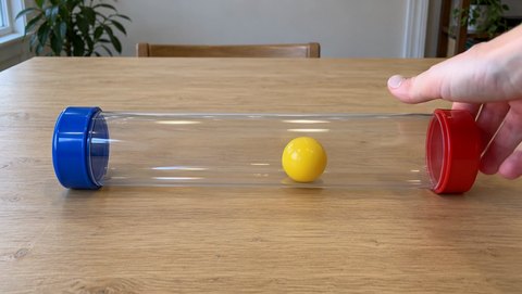
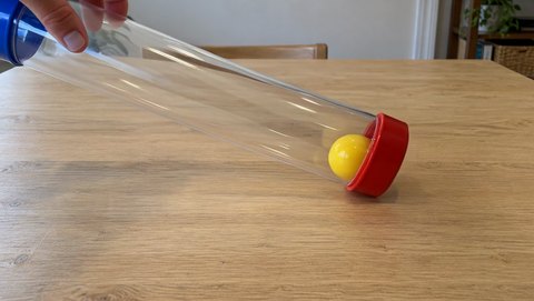
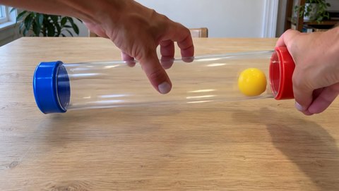
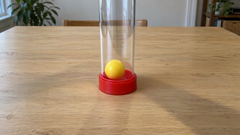
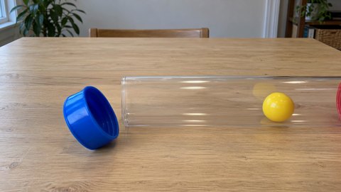
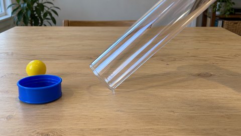
PAN 2 can also hold facts that the agent doesn’t know, and let the agent discover them through acting. A ball sits in a tube closed by two caps: a blue one that comes off, and a red one that is glued shut. The glue is invisible in the starting image; it is stated only in the text given to PAN 2, never to the agent. An LLM agent is asked to retrieve the ball from the tube. In each attempt, it proposes a short plan, PAN 2 simulates it, and the agent judges from the 5-second clip whether it has succeeded; if not, it tries again with all its previous plans, clips and judgements in view, in a setup similar to Reflexion.
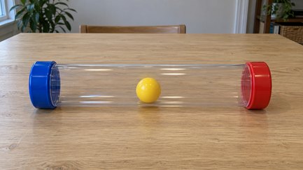
LLM agent ⇄ PAN 2· plan, 5-second simulation, review; every attempt starts from this image
Known only to the world model: the blue cap comes off; the red cap is glued shut.
- 1Pull red cap
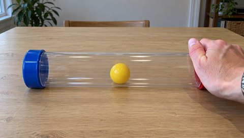
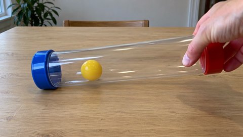 Ball still inside
- 2Twist red cap
 Reviewed as “cap off” (incorrect)
- 3Invert; shake
 Ball still inside
- 4Twist red; pinch
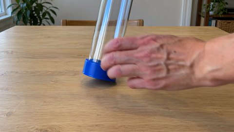
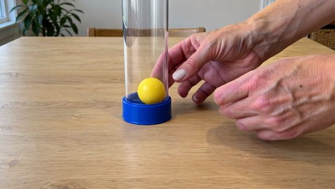 Ball still inside
- 5Pull red; shake
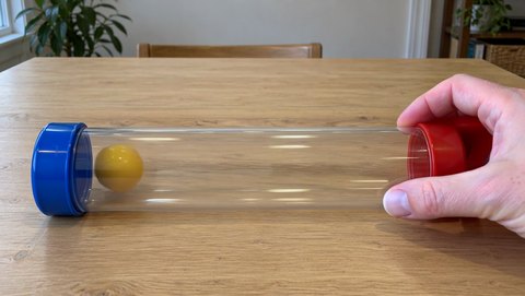
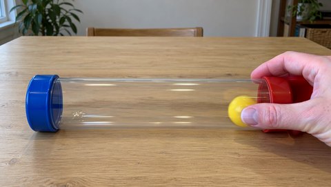 Ball still inside
- 6Remove blue cap
 Ball exits
The agent first pulls the red cap, then twists it. Misreading the second simulation, it concludes that the cap has come off, and spends its next three attempts trying to force the ball out of that end, whether it be inverting and shaking the tube, pinching and twisting the red cap, or pulling it again. On its sixth attempt, it turns to the blue cap, and the ball comes out. The agent learned a property of the world it could not see, through simulated interaction alone. In this case, the text-based state carries what the image cannot.
Next steps for agent learning
Two steps remain before agents can train in world simulation at scale. The first is a world that grows and stays consistent as the agent explores it, which is the subject of an upcoming post. This requires coordinated conceptual and perceptual memory built into the model, along with increasingly faithful simulations of action consequences. The second is training agents on experience gathered across simulated episodes, so that what they learn carries across tasks and ultimately improves decisions in the physical world.
Try PAN 2
Predicting the next word gave us models that reason with language. Likewise, we believe predicting the next world is how models will learn to reason about the physical world. PAN 2 is our step in that direction: a world model that reasons about what happens, renders how it unfolds, and gives agents a simulator to practice in before they act.
PAN 2 is open, with weights, training code and inference code. Try it on your own scenes, build on it, and tell us what you simulate, and where it breaks.
Open weight
Download the model weights from Hugging Face.

Training code
Inspect, finetune, or train your own model from scratch.

Inference code
Run PAN 2 with vLLM, HF Diffusers or FastVideo.


Citation
@misc{pan2026pan2,
  title        = {{PAN 2}: A Foundation World Model for Physical Intelligence},
  author       = {{PAN Team}},
  howpublished = {Technical blog, Institute of Foundation Models, MBZUAI},
  year         = {2026},
  month        = nov
}
References
1.Eric Xing, Mingkai Deng, and Jinyu Hou. Critique of World Model. 2025. Paper.
2.Esser et al. Scaling Rectified Flow Transformers for High-Resolution Image Synthesis. 2024. Paper.
3.Lipman et al. Flow Matching for Generative Modeling. ICLR, 2023. Paper.
4.Jianyuan Wang et al. VGGT-Ω. CVPR, 2026. Project and paper.
5.Jiazheng Xu et al. ImageReward: Learning and Evaluating Human Preferences for Text-to-Image Generation (ReFL). NeurIPS, 2023. Paper.
6.Jie Wu et al. RewardDance: Reward Scaling in Visual Generation. 2025. Paper.
7.Jiazheng Xu et al. VisionReward: Fine-Grained Multi-Dimensional Human Preference Learning for Image and Video Generation. Paper · Code.
8.Keller Jordan. Muon: An Optimizer for Hidden Layers in Neural Networks. 2024. Article.
9.Jingyuan Liu et al. Muon Is Scalable for LLM Training. 2025. Paper.
10.Saman Motamed et al. Do Generative Video Models Understand Physical Principles? 2025. Paper · Benchmark and Verified leaderboard.
11.NVIDIA et al. Cosmos 3: Omnimodal World Models for Physical AI. 2026. Paper · Official model reference.
12.Lightricks. LTX-2.5. 2026. Official model card · Code.
13.MiniMax. MiniMax-H3. 2026. Official repository · Model card.
14.Black Forest Labs. FLUX 3. 2026. Official announcement.
15.ByteDance Seed. Seedance 2.5. 2026. Official project page.
16.Yufan Deng et al. Rethinking Video Generation Model for the Embodied World (RBench). 2026. Paper · Benchmark and code.
17.Juyi Lin et al. PhyGround: Benchmarking Physical Reasoning in Generative World Models. 2026. Paper · Project.
18.Mitchell Wortsman et al. Model Soups: Averaging Weights of Multiple Fine-Tuned Models Improves Accuracy without Increasing Inference Time. ICML, 2022. Paper.
19.Alexandre Ramé et al. Rewarded Soups: Towards Pareto-Optimal Alignment by Interpolating Weights Fine-Tuned on Diverse Rewards. NeurIPS, 2023. Paper.
20.Noah Shinn et al. Reflexion: Language Agents with Verbal Reinforcement Learning. NeurIPS, 2023. Paper.